Read Directly from IIASA Data Resources

IIASA’s new scenario explorer is not only a great resource on its own, but it also allows the underlying datasets to be directly queried. pyam takes advantage of this ability to allow you to easily pull data and work with it.

import pyam
from pyam.iiasa import valid_connection_names

There are currently not many available data sources, but more will be added with time

valid_connection_names()

['iamc15']

In this example, we will be pulling data from the Special Report on 1.5C explorer. This can be done in a number of ways, for example

pyam.read_iiasa('iamc15')
pyam.read_iiasa_iamc15()

However, this would pull all available data. It is also possible to query specific subsets of data in a manner similar to pyam.IamDataFrame.filter(). We’ll do that to keep it manageable.

df = pyam.read_iiasa_iamc15(
    model='MESSAGEix*',
    variable=['Emissions|CO2', 'Primary Energy|Coal'],
    region='World'
)

INFO:root:You are connected to the iamc15 scenario explorer. Please cite as:

D. Huppmann, E. Kriegler, V. Krey, K. Riahi, J. Rogelj, S.K. Rose, J. Weyant, et al., IAMC 1.5°C Scenario Explorer and Data hosted by IIASA. IIASA & IAMC, 2018. doi: 10.22022/SR15/08-2018.15429, url: data.ene.iiasa.ac.at/iamc-1.5c-explorer

Here we pulled out all results for model(s) that start with ‘MESSAGEix’ that are in the ‘World’ region and associated with the two named variables.

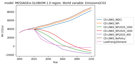
Let’s plot CO2 emissions.

ax = df.filter(variable='Emissions|CO2').line_plot(
    color='scenario',
    legend=dict(loc='center left', bbox_to_anchor=(1.0, 0.5))
)

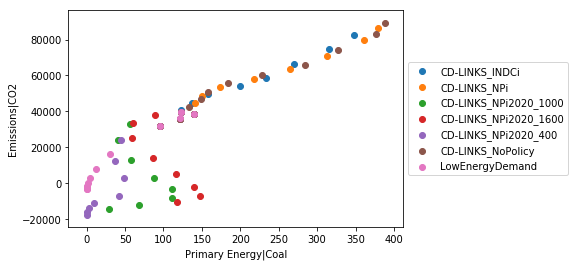
And now continue doing all of your analysis!

ax = df.scatter(
    x='Primary Energy|Coal',
    y='Emissions|CO2',
    color='scenario',
    legend=dict(loc='center left', bbox_to_anchor=(1.0, 0.5))
)

Exploring the Data Source

If you’re interested in what data is actually in the data source, you can use pyam.iiasa.Connection to do so.

conn = pyam.iiasa.Connection('iamc15')

INFO:root:You are connected to the iamc15 scenario explorer. Please cite as:

D. Huppmann, E. Kriegler, V. Krey, K. Riahi, J. Rogelj, S.K. Rose, J. Weyant, et al., IAMC 1.5°C Scenario Explorer and Data hosted by IIASA. IIASA & IAMC, 2018. doi: 10.22022/SR15/08-2018.15429, url: data.ene.iiasa.ac.at/iamc-1.5c-explorer

The conn object has a number of useful functions for listing what’s in the dataset. A few of them are shown below.

conn.models().head()

0        AIM/CGE 2.0
1        AIM/CGE 2.1
2      C-ROADS-5.005
3           GCAM 4.2
4    GENeSYS-MOD 1.0
Name: model, dtype: object

conn.scenarios().head()

0    ADVANCE_2020_1.5C-2100
1        ADVANCE_2020_Med2C
2         ADVANCE_2020_WB2C
3        ADVANCE_2030_Med2C
4    ADVANCE_2030_Price1.5C
Name: scenario, dtype: object

conn.variables().head()

0    AR5 climate diagnostics|Concentration|CO2|FAIR...
1    AR5 climate diagnostics|Concentration|CO2|MAGI...
2    AR5 climate diagnostics|Forcing|Aerosol|Direct...
3    AR5 climate diagnostics|Forcing|Aerosol|MAGICC...
4    AR5 climate diagnostics|Forcing|Aerosol|Total|...
Name: variable, dtype: object

conn.regions().head()

0          World
1         R5ASIA
2          R5LAM
3          R5MAF
4    R5OECD90+EU
Name: region, dtype: object

You can directly query the the conn, which will give you a pd.DataFrame

df = conn.query(
    model='MESSAGEix*',
    variable=['Emissions|CO2', 'Primary Energy|Coal'],
    region='World'
)
df.head()

	model	region	runId	scenario	time	unit	value	variable	version	year
0	MESSAGEix-GLOBIOM 1.0	World	238	CD-LINKS_INDCi	-1	Mt CO2/yr	31667.90819	Emissions|CO2	1	2000
1	MESSAGEix-GLOBIOM 1.0	World	238	CD-LINKS_INDCi	-1	Mt CO2/yr	35933.06970	Emissions|CO2	1	2005
2	MESSAGEix-GLOBIOM 1.0	World	238	CD-LINKS_INDCi	-1	Mt CO2/yr	38542.01816	Emissions|CO2	1	2010
3	MESSAGEix-GLOBIOM 1.0	World	238	CD-LINKS_INDCi	-1	Mt CO2/yr	39615.22255	Emissions|CO2	1	2020
4	MESSAGEix-GLOBIOM 1.0	World	238	CD-LINKS_INDCi	-1	Mt CO2/yr	40671.28065	Emissions|CO2	1	2030

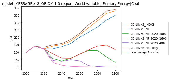
And you can easily turn this into a pyam.IamDataFrame to continue your analysis.

df = pyam.IamDataFrame(df)
ax = df.filter(variable='Primary Energy|Coal').line_plot(
    color='scenario',
    legend=dict(loc='center left', bbox_to_anchor=(1.0, 0.5))
)