First steps with the pyam package
An open-source Python package for IAM scenario analysis and visualization
Scope and feature overview
pyam package provides a range of diagnostic tools and
functionsAn illustrative example of the IAMC template is shown below; see data.ene.iiasa.ac.at/database/ for more information.
| Model | Scenario | Region | Variable | Unit | 2005 | 2010 | 2015 |
|---|---|---|---|---|---|---|---|
| MESSAGE V.4 | AMPERE3-Base | World | Primary Energy | EJ/y | 454.5 | 479.6 | … |
| … | … | … | … | … | … | … | … |
This notebook illustrates some basic functionality of the pyam
package and the IamDataFrame class:
- Importing timeseries data from
xlsxorcsvfiles. - Listing models, scenarios and variables included in the data.
- Display of timeseries data as pd.DataFrame.
- Visualization tools for timeseries data using the matplotlib package.
- Evaluating the model data and executing a range of diagnostic checks for identifying outliers.
- Categorization of scenarios according to timeseries data values or checks on required variables.
- Exporting data to
xlsxusing the IAMC template.
Tutorial data
The timeseries data used in this tutorial is a partial snapshot of the scenario database compiled for the IPCC’s Fifth Assessment Report (AR5):
Krey V., O. Masera, G. Blanford, T. Bruckner, R. Cooke, K. Fisher-Vanden, H. Haberl, E. Hertwich, E. Kriegler, D. Mueller, S. Paltsev, L. Price, S. Schlömer, D. Ürge-Vorsatz, D. van Vuuren, and T. Zwickel, 2014: Annex II: Metrics & Methodology.
In: Climate Change 2014: Mitigation of Climate Change. Contribution of Working Group III to the Fifth Assessment Report of the Intergovernmental Panel on Climate Change [Edenhofer, O., R. Pichs-Madruga, Y. Sokona, E. Farahani, S. Kadner, K. Seyboth, A. Adler, I. Baum, S. Brunner, P. Eickemeier, B. Kriemann, J. Savolainen, S. Schlömer, C. von Stechow, T. Zwickel and J.C. Minx (eds.)]. Cambridge University Press, Cambridge, United Kingdom and New York, NY, USA. Link
The complete database is publicly available at tntcat.iiasa.ac.at/AR5DB/.
The data snapshot used for this tutorial consists of selected data from two model intercomparison projects:
Energy Modeling Forum Round 27 (EMF27), see the Special Issue in Climatic Change 3-4, 2014.
EU FP7 project AMPERE, see the following scientific publications:
- Riahi, K., et al. (2015). “Locked into Copenhagen pledges — Implications of short-term emission targets for the cost and feasibility of long-term climate goals.” Technological Forecasting and Social Change 90(Part A): 8-23. DOI: 10.1016/j.techfore.2013.09.016
- Kriegler, E., et al. (2015). “Making or breaking climate targets: The AMPERE study on staged accession scenarios for climate policy.” Technological Forecasting and Social Change 90(Part A): 24-44. DOI: 10.1016/j.techfore.2013.09.021
Import package and load data from the AR5 tutorial snapshot
We import the snapshot timeseries data from the file
tutorial_AR5_data.csv in the tutorial folder.
As a first step, we show lists of all models, scenarios, regions, and the variables and units included in the snapshot.
In [1]:
import pyam
import pandas as pd
import matplotlib.pyplot as plt

%matplotlib inline
In [2]:
df = pyam.IamDataFrame(data='tutorial_AR5_data.csv', encoding='utf-8')
INFO:root:Reading `tutorial_AR5_data.csv`
In [3]:
df.models()
Out[3]:
0    AIM-Enduse 12.1
1           GCAM 3.0
2          IMAGE 2.4
3        MERGE_EMF27
4        MESSAGE V.4
5         REMIND 1.5
6        WITCH_EMF27
Name: model, dtype: object
In [4]:
df.scenarios()
Out[4]:
0             AMPERE3-450
1         AMPERE3-450P-CE
2         AMPERE3-450P-EU
3             AMPERE3-550
4         AMPERE3-550P-EU
5     AMPERE3-Base-EUback
6       AMPERE3-CF450P-EU
7          AMPERE3-RefPol
8          EMF27-450-Conv
9         EMF27-450-NoCCS
10       EMF27-550-LimBio
11    EMF27-Base-FullTech
12          EMF27-G8-EERE
Name: scenario, dtype: object
In [5]:
df.regions()
Out[5]:
0      ASIA
1       LAM
2       MAF
3    OECD90
4       REF
5     World
Name: region, dtype: object
In [6]:
df.variables(include_units=True)
Out[6]:
| variable | unit | |
|---|---|---|
| 0 | Emissions|CO2 | Mt CO2/yr |
| 1 | Emissions|CO2|Fossil Fuels and Industry | Mt CO2/yr |
| 2 | Emissions|CO2|Fossil Fuels and Industry|Energy... | Mt CO2/yr |
| 3 | Emissions|CO2|Fossil Fuels and Industry|Energy... | Mt CO2/yr |
| 4 | Price|Carbon | US$2005/t CO2 |
| 5 | Primary Energy | EJ/yr |
| 6 | Primary Energy|Coal | EJ/yr |
| 7 | Primary Energy|Fossil|w/ CCS | EJ/yr |
| 8 | Temperature|Global Mean|MAGICC6|MED | °C |
Tutorial on data filtering
A selection of the timeseries data of an IamDataFrame can be
obtained by applying the filter() funtion, which takes a dictionary
of filter criteria as argument. The function filter() returns a
filtered clone of the IamDataFrame.
Filtering by model names, scenarios and regions
The feature for filtering by model, scenario or region are
implemented using exact string matching, where * can be used as a
wildcard:
Applying the keyword argument filter
model='MESSAGE'to theIamDataFramewill return an empty array.Filtering for
model='MESSAGE*'will return all scenarios from the “MESSAGE” family, identified by the model name “MESSAGE” and a version identifier.
In [7]:
df.filter(model='MESSAGE').models()
WARNING:root:Filtered IamDataFrame is empty!
Out[7]:
Series([], Name: model, dtype: object)
In [8]:
df.filter(model='MESSAGE*')[['model', 'scenario']].drop_duplicates()
Out[8]:
| model | scenario | |
|---|---|---|
| 386 | MESSAGE V.4 | AMPERE3-450 |
| 392 | MESSAGE V.4 | AMPERE3-450P-EU |
| 398 | MESSAGE V.4 | AMPERE3-550 |
| 404 | MESSAGE V.4 | AMPERE3-RefPol |
| 410 | MESSAGE V.4 | EMF27-550-LimBio |
| 434 | MESSAGE V.4 | EMF27-Base-FullTech |
Using keyword keep=False allows you to discard everything that is
found by the filter rather than keeping it
In [9]:
df.filter(region="World", keep=False).regions()
Out[9]:
0      ASIA
1       LAM
2       MAF
3    OECD90
4       REF
Name: region, dtype: object
In [10]:
df.filter(region="World", keep=True).regions()
Out[10]:
0    World
Name: region, dtype: object
Filtering by variables and hierarchy levels
Filtering for variable strings works in an identical way as above,
with * available as a wildcard.
Filtering for Primary Energy will return only exactly those data.
Filtering for _Primary Energy|*_ will return all sub-categories of primary-energy level (and only the sub-categories).
In additon, IAM variables can be filtered by the level, i.e., the
“depth” of the variable in a hierarchical reading of the string
separated by '|'. That is, the variable Primary Energy has level
0, while Primary Energy|Coal has level 1. Filtering by both
variables and level will search for the hierarchical depth
following the variable string, so filter arguments
'variable': 'Primary Energy|*' and 'level': 0 will return all
variables immediately below 'Primary Energy'. Filtering by level
only will return all variables at that depth.
'Emissions' variable.'Emissions|'; the list returned by the function call will include
only 'Emissions|CO2|Fossil Fuels and Industry', because the level
argument (by default) only shows variables at exactly the hierarchical
levels below 'Emissions|...'.The third example illustrates another use case of the level argument -
filtering by '1-' instead of 1 will return all variables up to
the specified depth.
The last cell shows how to filter only by hierarchical level, without
providing a variable string. The function returns all variables that are
at the top hierarchical level (i.e., 'Primary Energy') and those at
the first sub-category level. Keep in mind that there are no variables
'Emissions' or 'Price' (no top level).
In [11]:
df.filter(variable='Emissions|*').variables()
Out[11]:
0                                        Emissions|CO2
1              Emissions|CO2|Fossil Fuels and Industry
2    Emissions|CO2|Fossil Fuels and Industry|Energy...
3    Emissions|CO2|Fossil Fuels and Industry|Energy...
Name: variable, dtype: object
In [12]:
df.filter(variable='Emissions|*', level=1).variables()
Out[12]:
0    Emissions|CO2|Fossil Fuels and Industry
Name: variable, dtype: object
In [13]:
df.filter(variable='Emissions|*', level='1-').variables()
Out[13]:
0                              Emissions|CO2
1    Emissions|CO2|Fossil Fuels and Industry
Name: variable, dtype: object
In [14]:
df.filter(level='1-').variables()
Out[14]:
0          Emissions|CO2
1           Price|Carbon
2         Primary Energy
3    Primary Energy|Coal
Name: variable, dtype: object
Filtering by year
range.range(2010,2015) is interpreted as
[2010, 2011, 2012, 2013, 2014].Getting help
When in doubt, you can look at the help for any function by appending it
with a ?.
In [15]:
df.filter?
Displaying timeseries data
As a next step, we want to view a selection of the data in the tutorial
snapshot using the IAMC standard. The timeseries() function returns
the data in the standard IAMC format as a pd.DataFrame.
In [16]:
(df
 .filter(scenario='AMPERE3-450', variable='Primary Energy|Coal', region='World')
 .timeseries()
)
Out[16]:
| 2005 | 2010 | 2020 | 2030 | 2040 | 2050 | 2060 | 2070 | 2080 | 2090 | 2100 | |||||
|---|---|---|---|---|---|---|---|---|---|---|---|---|---|---|---|
| model | scenario | region | variable | unit | |||||||||||
| GCAM 3.0 | AMPERE3-450 | World | Primary Energy|Coal | EJ/yr | 120.76 | 144.95 | 176.44 | 204.42 | 212.84 | 186.02 | 138.23 | 106.98 | 82.44 | 36.55 | 14.89 |
| IMAGE 2.4 | AMPERE3-450 | World | Primary Energy|Coal | EJ/yr | 111.62 | 138.69 | 148.60 | 121.24 | 102.62 | 101.41 | 111.41 | 138.40 | 181.03 | 224.03 | 264.77 |
| MESSAGE V.4 | AMPERE3-450 | World | Primary Energy|Coal | EJ/yr | 121.12 | 138.09 | 119.94 | 93.11 | 52.07 | 71.91 | 98.09 | 127.76 | 136.08 | 108.49 | 41.21 |
| REMIND 1.5 | AMPERE3-450 | World | Primary Energy|Coal | EJ/yr | 122.20 | 135.47 | 92.72 | 45.87 | 22.33 | 20.39 | 16.64 | 12.35 | 5.94 | 2.36 | 1.77 |
For displaying data in a different format, the class IamDataFrame
has a wrapper of the pd.DataFrame.pivot_table() function. It allows
to flexibly specify the columns and rows. The function automatically
aggregates by summation or counting (specified by the parameter
aggfunc) over all timeseries data identifiers (‘model’, ‘scenario’,
‘variable’, ‘region’, ‘unit’, ‘year’) which are not used as index or
columns.
In the example below, the filter of the timeseries data is set for all subcategories of ‘Primary Energy’, which are then summed up in the displayed table.
In [17]:
(df
 .filter(variable='Primary Energy', region='World')
 .pivot_table(index=['year'], columns=['scenario'], values='value', aggfunc='sum')
)
Out[17]:
| scenario | AMPERE3-450 | AMPERE3-450P-CE | AMPERE3-450P-EU | AMPERE3-550 | AMPERE3-550P-EU | AMPERE3-Base-EUback | AMPERE3-CF450P-EU | AMPERE3-RefPol | EMF27-450-Conv | EMF27-450-NoCCS | EMF27-550-LimBio | EMF27-Base-FullTech | EMF27-G8-EERE |
|---|---|---|---|---|---|---|---|---|---|---|---|---|---|
| year | |||||||||||||
| 2005 | 1821.09 | 1366.48 | 1821.09 | 1818.71 | 464.82 | 922.58 | 925.23 | 1818.44 | 2234.35 | 1381.84 | 3130.81 | 3130.60 | 868.79 |
| 2010 | 1972.13 | 1492.28 | 1972.02 | 1969.57 | 514.07 | 1015.78 | 1018.44 | 1969.50 | 2504.99 | 1542.90 | 3457.08 | 3459.28 | 985.16 |
| 2020 | 2253.49 | 1787.40 | 2399.41 | 2322.23 | 611.34 | 1258.24 | 1262.07 | 2401.37 | 2428.61 | 1424.26 | 3781.16 | 4135.65 | 947.08 |
| 2030 | 2530.95 | 2101.60 | 2863.85 | 2670.22 | 734.11 | 1532.12 | 1536.54 | 2869.96 | 2545.94 | 1470.64 | 4057.28 | 4846.37 | 933.08 |
| 2040 | 2795.47 | 2206.09 | 2940.96 | 3000.37 | 789.70 | 1802.62 | 1574.14 | 3305.70 | 2698.99 | 1670.51 | 4355.16 | 5588.19 | 1007.83 |
| 2050 | 3064.07 | 2348.02 | 3087.59 | 3312.70 | 815.79 | 2104.63 | 1652.02 | 3709.45 | 2759.41 | 1794.47 | 4586.40 | 6353.16 | 1075.16 |
| 2060 | 3321.63 | 2537.42 | 3317.84 | 3532.21 | 861.79 | 2359.38 | 1774.56 | 4056.44 | 2198.22 | 1257.99 | 4164.92 | 6172.01 | 531.36 |
| 2070 | 3512.57 | 2683.30 | 3526.56 | 3722.65 | 901.57 | 2564.68 | 1912.48 | 4391.18 | 2240.64 | 1344.42 | 4430.28 | 6768.95 | 563.62 |
| 2080 | 3689.77 | 2824.81 | 3724.06 | 3926.94 | 943.47 | 2708.68 | 2033.99 | 4700.20 | 2256.69 | 1461.97 | 4690.79 | 7288.74 | 568.90 |
| 2090 | 3946.92 | 3025.65 | 3962.55 | 4120.64 | 964.16 | 2775.73 | 2190.16 | 4959.63 | 2259.28 | 1576.82 | 4965.55 | 7653.56 | 550.30 |
| 2100 | 4263.04 | 3281.83 | 4272.05 | 4387.84 | 1005.66 | 2879.44 | 2403.99 | 5217.67 | 2246.02 | 1729.13 | 5188.70 | 7983.73 | 563.39 |
If you are familiar with the python package pandas, you can use
many of usual functions directly on the IamDataFrame. The function
head(), for example, will show the first n rows of the data in
long form (columns are in year/value format).
In [18]:
df.head()
Out[18]:
| model | scenario | region | variable | unit | year | value | |
|---|---|---|---|---|---|---|---|
| 0 | AIM-Enduse 12.1 | EMF27-450-Conv | ASIA | Emissions|CO2 | Mt CO2/yr | 2005 | 10540.74 |
| 3 | AIM-Enduse 12.1 | EMF27-450-Conv | LAM | Emissions|CO2 | Mt CO2/yr | 2005 | 3285.00 |
| 6 | AIM-Enduse 12.1 | EMF27-450-Conv | MAF | Emissions|CO2 | Mt CO2/yr | 2005 | 4302.21 |
| 9 | AIM-Enduse 12.1 | EMF27-450-Conv | OECD90 | Emissions|CO2 | Mt CO2/yr | 2005 | 12085.85 |
| 12 | AIM-Enduse 12.1 | EMF27-450-Conv | REF | Emissions|CO2 | Mt CO2/yr | 2005 | 3306.95 |
Visualization of timeseries
pyam package.plotting.ipynb notebook for a full tutorial on
plotting.
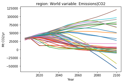
In [19]:
df.filter(variable='Emissions|CO2', region='World').line_plot(legend=False)
Out[19]:
<matplotlib.axes._subplots.AxesSubplot at 0x7fc6af427588>
Validation and diagnostic assessment of timeseries data
When analyzing scenario results, it is often useful to check whether certain timeseries exist or the values are within a specific range. For example, it may make sense to ensure that reported data for historical periods are close to established reference data or that near-term developments are reasonable.
The following section provides three illustrations: 1. Check whether a
timeseries 'Primary Energy' exists in each scenario (in at least one
year). 2. Check for every scenario whether the value for
'Primary Energy' at the global level exceeds 515 EJ/y in the
reference year 2010 (the value must satisfy an upper bound of 515 EJ/y
in this notation). 3. Check for every scenario from the AMPERE
project whether the value for 'Primary Energy|Coal' exceeds 400 EJ/y
in mid-century.
validate() function takes a filters dictionary to perform
the checks on a selection of models/scenarios similar to the functions
introduced above.criteria argument can specify a valid range by an upper and
lower bound (up, lo) for a variable and a subset of years to
which the validation is applied - all scenarios with a value in at
least one year outside that range are considered to not satisfy the
validation.By setting the argument exclude=True, all scenarios failing the
validation will be categorized as exclude in the metadata. This
allows to remove these scenarios from subsequent analysis or figures.
In [20]:
df.require_variable(variable='Primary Energy')
INFO:root:All scenarios have the required variable `Primary Energy`
In [21]:
df.validate(criteria={'Primary Energy': {'up': 515, 'year': 2010}})
INFO:root:9 of 6622 data points to not satisfy the criteria
Out[21]:
| model | scenario | region | variable | unit | year | value | |
|---|---|---|---|---|---|---|---|
| 678 | AIM-Enduse 12.1 | EMF27-450-Conv | World | Primary Energy | EJ/yr | 2010 | 518.89 |
| 701 | AIM-Enduse 12.1 | EMF27-450-NoCCS | World | Primary Energy | EJ/yr | 2010 | 518.81 |
| 724 | AIM-Enduse 12.1 | EMF27-550-LimBio | World | Primary Energy | EJ/yr | 2010 | 518.81 |
| 747 | AIM-Enduse 12.1 | EMF27-Base-FullTech | World | Primary Energy | EJ/yr | 2010 | 518.81 |
| 770 | AIM-Enduse 12.1 | EMF27-G8-EERE | World | Primary Energy | EJ/yr | 2010 | 518.64 |
| 1181 | REMIND 1.5 | EMF27-450-Conv | World | Primary Energy | EJ/yr | 2010 | 519.64 |
| 1202 | REMIND 1.5 | EMF27-450-NoCCS | World | Primary Energy | EJ/yr | 2010 | 519.64 |
| 1223 | REMIND 1.5 | EMF27-550-LimBio | World | Primary Energy | EJ/yr | 2010 | 519.64 |
| 1244 | REMIND 1.5 | EMF27-Base-FullTech | World | Primary Energy | EJ/yr | 2010 | 519.64 |
In [22]:
pyam.validate(df,
              filters={'region': 'World', 'scenario': 'AMPERE*'},
              criteria={'Primary Energy|Coal': {'up': 400, 'year': 2050}}
)
`filters` keyword argument in filters() is deprecated and will be removed in the next release
INFO:root:1 of 1566 data points to not satisfy the criteria
Out[22]:
| model | scenario | region | variable | unit | year | value | |
|---|---|---|---|---|---|---|---|
| 3432 | GCAM 3.0 | AMPERE3-Base-EUback | World | Primary Energy|Coal | EJ/yr | 2050 | 424.09 |
Categorization of scenarios by timeseries characteristics
It is often useful to apply categorization to classes of scenarios according to specific characteristics of the timeseries data. In the following example, we use the temperature change assessment by MAGICC 6 to group scenarios by the median global warming by the end of the century (year 2100).
We proceed in the following steps:
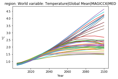
- Plot the timeseries data of the variable that we want to use. This provides some insights on useful thresholds for the categorization.
- Use the function
categorize()to apply a categorization (and colour code for later use) to all scenarios that satisfy a number of specific criteria. - Use the categorization of scenarios for analysis of other timeseries data.
In [23]:
v = 'Temperature|Global Mean|MAGICC6|MED'
df.filter(region='World', variable=v).line_plot(legend=False)
Out[23]:
<matplotlib.axes._subplots.AxesSubplot at 0x7fc6af309a20>
We now use the categorization feature of the pyam package to group
scenarios by temperature outcome by the end of the century.
The first cell sets the 'Temperature' categorization to the default
"uncategorized". This is not necessary per se (setting a meta column
via the categorization will mark all non-assigned rows as
"uncategorized" (if the value is a string) or np.nan. Still,
having this cell may be helpful in this tutorial if you are going back
and forth between cells to reset the assignment.
The function categorize() takes color and similar arguments,
which can then be used by the plotting library.
In [24]:
df.set_meta(meta='uncategorized', name='Temperature')
In [25]:
df.categorize(
    'Temperature', 'Below 1.6C',
    criteria={v: {'up': 1.6, 'year': 2100}},
    color='cornflowerblue'
)
INFO:root:4 scenarios categorized as `Temperature: Below 1.6C`
In [26]:
df.categorize(
    'Temperature', 'Below 2.0C',
    criteria={'Temperature|Global Mean|MAGICC6|MED': {'up': 2.0, 'lo': 1.6, 'year': 2100}},
    color='forestgreen'
)
INFO:root:8 scenarios categorized as `Temperature: Below 2.0C`
In [27]:
df.categorize(
    'Temperature', 'Below 2.5C',
    criteria={v: {'up': 2.5, 'lo': 2.0, 'year': 2100}},
    color='gold'
)
INFO:root:16 scenarios categorized as `Temperature: Below 2.5C`
In [28]:
df.categorize(
    'Temperature', 'Below 3.5C',
     criteria={v: {'up': 3.5, 'lo': 2.5, 'year': 2100}},
     color='firebrick'
)
INFO:root:3 scenarios categorized as `Temperature: Below 3.5C`
In [29]:
df.categorize(
    'Temperature', 'Above 3.5C',
    criteria={v: {'lo': 3.5, 'year': 2100}},
    color='magenta'
)
INFO:root:9 scenarios categorized as `Temperature: Above 3.5C`
Two models included in the snapshot have not been assessed by MAGICC6
regarding their long-term climate and warming impact. Therefore, the
timeseries 'Temperature|Global Mean|MAGICC6|MED' does not exist, and
they have not been categorized.
In [30]:
df.require_variable(variable=v, exclude_on_fail=False)
INFO:root:8 scenarios do not include required variable `Temperature|Global Mean|MAGICC6|MED`
Out[30]:
| model | scenario | |
|---|---|---|
| 0 | AIM-Enduse 12.1 | EMF27-450-Conv |
| 1 | AIM-Enduse 12.1 | EMF27-450-NoCCS |
| 2 | AIM-Enduse 12.1 | EMF27-550-LimBio |
| 3 | AIM-Enduse 12.1 | EMF27-Base-FullTech |
| 4 | AIM-Enduse 12.1 | EMF27-G8-EERE |
| 5 | WITCH_EMF27 | EMF27-450-Conv |
| 6 | WITCH_EMF27 | EMF27-550-LimBio |
| 7 | WITCH_EMF27 | EMF27-Base-FullTech |
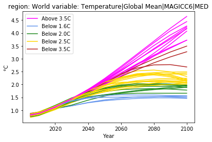
Now, we again display the median global temperature increase for all scenarios, but we use the colouring by category to illustrate the common charateristics across scenarios.
In [31]:
df.filter(variable='Temperature*').line_plot(color='Temperature', legend=True)
Out[31]:
<matplotlib.axes._subplots.AxesSubplot at 0x7fc6ac1a7f98>
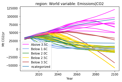
As a last step, we display the aggregate CO2 emissions by category. This allows to highlight alternative pathways within the same category.
In this step, we also export this figure as a png using the option
savefig. The figure will be saved in the tutorials folder.
In [32]:
fig, ax = plt.subplots()
(df
 .filter(variable='Emissions|CO2', region='World')
 .line_plot(ax=ax, color='Temperature', legend=True)
)
fig.savefig('co2_emissions.png')
Exporting timeseries data for further analysis
xlsx and csv in
the standard IAMC format.
In [33]:
df.to_excel('tutorial_export.xlsx')
df.export_metadata('tutorial_metadata.xlsx')